
Basic Operation
Step 1: Introduction
This tutorial provides a broad overview of how to use Genome Workbench to analyze and display data. Before beginning this tutorial, download and install Genome Workbench from the download page.
Step 2: Startup
When Genome Workbench starts up, the Main Application Window appears with several different panes. The Project Tree View is on the left and it's empty upon startup. This is where data you load, analyses you do and views you create will be stored.
The Main Application Window has many views and is completely configurable. You can click on a particular view and drag it where you want it. You can also stack views so they appear and folder tabs like the Event View and Task View shown below. When you click on a view to move it, you'll see icons showing the docking options for the view and by dropping the view on your choice, the view will move. Genome Workbench remembers your configuration so you only have to do this once.

Step 3: Using Search
To start, let's search for some data in the public databases at NCBI. Select the Search view from the Main Application Window. The Search View provides a single interface for many of the most frequent kinds of searches done in Genome Workbench.
The Search View is also accessible from the main menu as Tools -> Search or from the tool bar by clicking on the binoculars.
This view is also accessible from the main menu as File -> Search -> NCBI Public Databases. The view can be obtained also from View -> Search, and from the toolbar by clicking on the binoculars icon.
Let's now search for the gene superoxide dismutase in the Entrez Gene database. To do this, follow the steps below:
- Make sure the Search Tool in the Search View says: Search NCBI Public Databases
- Select Entrez Gene for the NCBI Database.
- Enter the gene name superoxide dismutase in the search dialog.
- Press the Enter key or click the Start button.

Step 4: Search for Genes (cont'd)
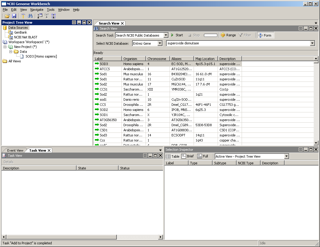
You should see a set of results like the those shown below. You can adjust the width of the columns by clicking on the divider between the column headings. If you right-click in the column header, you can choose to turn some columns on/off.

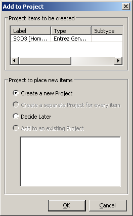
Select the item in the list corresponding to the human variant (Organism is Homo sapiens and the Label is SOD1 - might take a bit to find it) and right-click. Choose Add to Project from the contextual menu. You should see a dialog like the one to the right. The Entrez Gene database formats an object that contains a wealth of information about the gene and its placement on various assemblies. All of these are available to Genome Workbench.
Click OK in the dialog to create a new project. We will use the defaults from this dialog. In the future, you have the option to add this it to an existing project, or change how the it appears in the project tree.
Step 5: Viewing your data
Once the project is loaded, the main window should look something like the image below. The workspace area should now contains a blue notebook for the workspace and a green notebook for a project.
Genome Workbench organizes your data into workspaces and projects. Workspaces are small data files that point to projects; projects are files that contain data. A project can be shared between several workspaces. In addition, both projects and workspaces can hold separate notes and descriptors - a project can contain notes about how the project was created, what analyses were run and when, and what sorts of editing operations were performed.
Let's now take a look at this data. To open a view, select the data in the project tree and right-click and choose Open View . You could also choose View->Open View from the menu bar or double-click data. When the dialog appears choose Graphical View.
Genome Workbench will now ask you which sequence you wish to view. As mentioned previously, the Entrez Gene object holds references to many sequences in many different placements for each gene. You should see a dialog like the one on the right, asking you which sequence you want to view. We will start by looking at the placement of the gene on the reference chromosome. This sequence can be identified using the description column in the dialog. In addition, it can be identified through patterns of accessions:

- Accessions beginning with NC_ are reference sequence chromosomes
- Accessions beginning with NT_ are reference sequence contigs
- Accessions beginning with NG_ are reference sequences that have had some degree of human curation.
- Accessions beginning with NM_ are reference sequence mRNAs.
- Accessions beginning with NP_ are reference sequence proteins.
As you start using views, Genome Workbench will remember the views you've used most recently and present them to you in a shorter menu.
Step 6: The Graphical View
The graphical view shows the public annotations on a sequence, using both color and arrangement to show the relationships. In the view below, different annotations are shown with different colors:
- Green bars represent genes.
- Blue bars represent transcripts / mRNAs.
- Red bars represent coding regions / proteins.
At the bottom of the graphical view there are several controls. The content drop down is highlighted in the figure below and the SNP and the STS tracks are turned on.
In addition to the Central Dogma annotations, there are additional annotations that are available. These include:
- At the top of the image is a row of short blue tick marks. These represent variations from dbSNP for this sequence. As you zoom in and out, these will become available as selectable things.
- Just beneath the variations are a set of blue bars representing the components that are used to assemble this sequence. Most large genomic sequences are split into many smaller pieces and reassembled from these chunks; the blue bars show you where the chunk boundaries are, and what the approximate overlap between chunks is.
- Many other features, including sequence tagged sites (STSs, visible in the image below) are shown as black bars underneath the genes and gene products.

Step 7: Navigating in the Graphical View
There are several ways to zoom in and out in the graphical view. One way, shown below, uses a zoom slider. To show the zoom slider, press and hold the Z key; you can then zoom in and out by left-clicking and dragging the mouse up and down. The view will then change the level of zoom in real time.

You can also pan the view from left to right by left-clicking, and dragging from left to right.

A third way to zoom in is called rectangular or regional zoom. This is available by holding down the R key, left-clicking, and dragging over a region. When you do this, you will see a view like the one to the right. Try this now to zoom in to a region around an exon, as shown to the right.
Step 8: Zoomed In Detail
The Graphical View balances the depth of detail with the depth of zoom. As you zoom in more and more, you will see more and more detail. In the image below, the view is zoomed all the way in to the actual sequence. The gray sequence bars across the top are now duplicated, showing both the forward and reverse (complemented) strand of the chromosomal sequence. In addition, inside the protein coding region, the letters of the protein are inscribed, spaced out to account for the codon boundaries and reading frame. 
If you select a coding region annotation, you will see inscribed beneath each amino acid residue the letters of the codon actually responsible for that amino acid. The image below shows this.
If you hover over an annotation or over the gray sequence bars, you will receive a tool tip popup providing additional information. The images to the right show two tool tips - one over a feature, showing information about the feature as well as the GenBank display for this feature, and one for the sequence, providing details both about the organism involved and the location over which the mouse is positioned.
Step 9: Graphical View Configuration
The graphical view supports a wide range of visual customizations to make it easier to understand the data presented. The controls for customization are at the bottom of the graphical view (highlighted in the image on the below). And each track can be customized (also highlighted in the image below). The track controls will appear when you mouse over the title bar.
Among the things you can change are:
- Decorations. Annotations such as mRNA and coding region features can be displayed with a wide variety of decorations, such as circle or square anchors, arrow fletchings, and different kinds of arrow heads.
- Spacing. For many displays, a more compact display is preferred; to access this, choose the Compact option for spacing.
- Content. In many cases, you may be interested in seeing just a subset of features. The Content drop-down menu lets you choose what kinds of features to show; for example, the MolBio option shows just genes, mRNAs, and coding region annotations.
- Track Order. To change the order of the tracks, click in the track's title bar and drag.
The graphical view will remember your settings, so that the next time you create a graphical view, your settings will apply. This is true even if you exit Genome Workbench. In addition, you can create and save several different Themes of settings and easily switch back and forth between styles without having to remember a lot of settings.

Step 10: Launching Tools from the Graphical View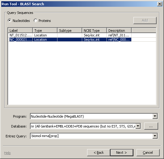

In the graphical view, everything you see is selectable, and you can perform actions on things you select. To select an item, just click on it and the object will highlight.
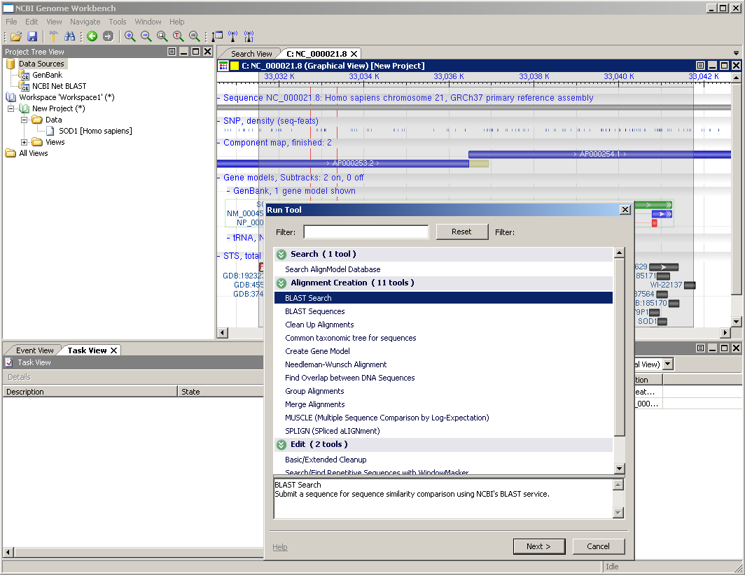
Let's run a BLAST search on a sequence in the graphical view. There is one gene annotated here: SOD1. Select a region of the genome containing this by clicking in the ruler above the sequence and dragging a gray rectangle to cover the gene model. Then, from the main menu, choose Tools -> Run Tool and the Run Tool dialog will appear. This tool will submit the sequence to the NCBI BLAST service for alignment against a set of sequences. When you choose this option, you should see a dialog like the one to the right.

There may be more than one sequence listed in the dialog, go ahead and choose the one whose label starts with NC_000021.8.
For this particular example, there are a couple things to change. First, let's choose MegaBLAST from the Program menu. Second, enter an Entrez query biomol mrna[prop] ensures that we're considering only those molecules known to be mRNAs.
Click Next.
There are many parameters that can be changed for BLAST, we're going to accept the defaults. Select these options and click Next.
Click Next.
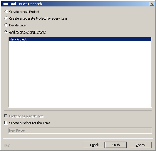
There are many options regarding the results. We'll simply add thisto the existing project.
Click Finish.
Once the sequence has been submitted, it will be entered into the BLAST polling systemfor retrieval. The Task View will help you track your job's progress.

Step 11: Viewing Results
When our alignment job is finished, the data will be added to the Graphical View automatically. Also, our Alignment will be added to the Project Tree View
In this view mismatches in alignments are colored red and insertions are blue.
Incidentally, you can arrange the data in the Data folder. If you select the folder, then right-click (or control-click for Mac OS), you will find options in the context menu to create a new folder. You can then cut and paste or drag-and-drop it into new locations. As you collect more and more results in a project, these folders will help you keep track of what each set of results means.

Step 12: Manipulating Alignments
The graphical view shows the newly obtained BLAST alignments as a set of disconnected bars hanging underneath our models. While this gives us some idea of regions of the genome that likely provide coding potential, it also confuses the issue significantly. Genome Workbench provides a couple of tools to make this visualization easier.

First, let's clean the alignment up, using the alignment cleaning tool at Tools -> Run Tool. This tool provides two algorithms for removing redundancies in alignments and for stringing disconnected pieces together. The tools are:
- The HitFilter is generally a good choice for working with large genomic alignments
- The Alignment Manager option is generally the best option for dealign with short, detailed alignments.
Let's choose the Alignment Manager option from the drop down and click Next. Then choose Add to an exisiting project and click Finish. The graphical view will change to look like the image below, and a new item will appear in the project tree.

Step 13: Finished
Congratulations, you completed the first tutorial!
In this tutorial, we examined several aspects of how Genome Workbench lets you work with data. These include:
- Searching for data using NCBI public databases such as Entrez Gene.
- Exploring projects in the workspace explorer portion of the Genome Workbench interface
- Creating and navigating in views such as the graphical view.
- Running analyses such as creating alignments of sets of sequences.
In all of these explorations, there are some common themes that will help you get the most out of Genome Workbench. These include:
- Use of context menus. If you right click (or control-click in Mac OS) on a view or on a selection somewhere, you will receive information about that object, including things that can be done to that object.
- Customization. No one set of view settings is correct for everyone. Genome Workbench contains some easy ways to customize each view so that the views can provide you with more information and more relevant information.
- Selections. Things you see on the screen are selectable, whether they are annotations on sequence, rows of an alignment, or swaths of sequence themselves. Genome Workbench uses selections as inputs to analyses.
Download
Current Version is 2.6.0 (released August 31, 2012)
- Release Notes
- Windows
- Mac OS X
- Linux (Ubuntu 10.04 LTS (Lucid Lynx))
- Source
- Older Versions